How to use pgfplots table in Latex

A few commonly used methods to construct tables in latex.

Table loading methods

1. Load a table through reading inline data

Example 1

\pgfplotstabletypeset[
	col sep=&,	% specify the column separation character
	row sep=\\,	% specify the row separation character
	columns/E/.style={string type} % specify the type of data in the designated column
]{
	A & B & C & D & E \\
	1 & 10 & 0.1 & 1000 & 2011-01-01 \\
	2 & 20 & 0.2 & 2000 & 2012-02-02 \\
	3 & 30 & 0.3 & 3000 & 2013-03-03 \\
	4 & 40 & 0.4 & 4000 & 2014-04-04 \\
	5 & 50 & 0.5 & 5000 & 2015-05-05 \\
}

• \pgfplotstabletypeset [<format>] {<inline data>}
• col sep = {<character>}
• row sep = {<character>}
• columns/{<column name>}/.style = {<type>}

Output:

2. Load a table through reading file

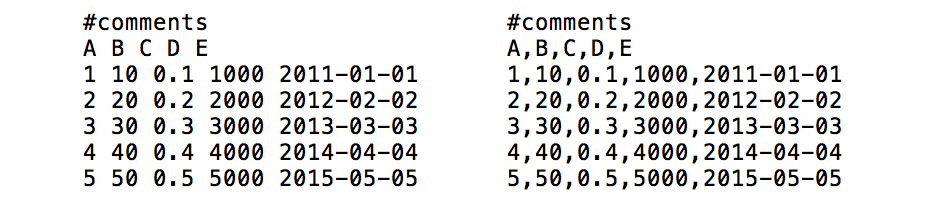
The following screenshot shows file “example.dat” and file “example.csv”.

Example 2(a)

\pgfplotstabletypeset[
	col sep=space,
	columns/E/.style={string type}
]{example.dat}

\pgfplotstabletypeset[
	col sep=comma,
	columns/E/.style={string type}
]{example.csv}

• \pgfplotstabletypeset [<format>] {<file name>}
• Lines starting with # in files are considered to be comment lines and are ignored

Outputs are exactly the same as the output in Example 1.

Example 2(b)

Load a table such that the output table only contains several specific columns.

\pgfplotstabletypeset[
	columns={A,B,D}	% specify the columns in output table
]{example.dat}

• columns={<cloumn name>,<column name>,···}

Output:

Example 2(c)

Load a table such that the output table only contains several specific rows.

\pgfplotstabletypeset[
	col sep=comma,
	columns/E/.style={string type},
	skip rows between index={0}{2},
	skip rows between index={4}{5}
]{example.csv}

• skip rows between index = {<begin>} {<end>}

Output:

Example 2(d)

Load a table without column names line in the text file.

The following screenshot shows file “example2.dat”. The first line in this file is not the column names line.

\pgfplotstabletypeset[
	col sep=space,
	columns/0/.style={column name=A},		% rename the column with index 0
	columns/1/.style={column name=B},
	columns/2/.style={column name=C},
	columns/3/.style={column name=D}
]{example_2.dat}

• columns/<column name> or <column index>/.style = {column name = <character>}

Output:

Row and Column formatting methods

Example 3(a)

Style the first row, last row, first column, last column and any designated column.

\pgfplotstabletypeset[
	col sep=comma,
	columns/E/.style={string type},
	column type=l,	% specify the align method
	every head row/.style={before row=\hline,after row=\hline},	% style the first row
	every last row/.style={after row=\hline},	% style the last row
	every first column/.style={column type/.add={|}{}},	% style the first column
	every last column/.style={column type/.add={}{|}},	% style the last column
	columns/C/.style = {column type/.add={|}{|}}	% style the designated column
]{example.csv}

• column type = r/l/c: align right, left or center.
• every head row/.style = {}, every last row/.style = {}, every first column/.style = {}, every last column/.style = {}
• before row = {<TEX code>}, after row = {<TEX code>}: contain TEX code which will be installed before the first cell in a row or after the last cell in a row.
• column type/.add={<before>}{<after>}
• columns/<column name>/.style = {}

Output:

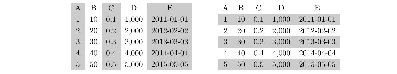
Example 3(b)

Style all the even(or odd) columns(or rows).

\pgfplotstabletypeset[
	col sep=comma,
	columns/E/.style={string type},
	every even column/.style={column type/.add={>{\columncolor[gray]{.8}}}{}}
]{example.csv}

\pgfplotstabletypeset[
	col sep=comma,
	columns/E/.style={string type},
	every even row/.style={before row={\rowcolor[gray]{.8}}}
]{example.csv}

• every even column/.style = { }, every odd column/.style = { } (Index starts with 0).
• every even row/.style = { }, every odd row/.style = { } (The first row is supposed to be a “head” row and does not count. Indexing starts with 0).

Output:

Example 3(c)

Using math expression to assign contents for designated column.

\pgfplotstabletypeset[
	col sep=comma,
	columns/E/.style={string type},
	columns/A/.style={
		column name={$\text{A}\times5$},
		preproc/expr={5*##1}
		}
]{example.csv}

• columns/<column name>/.style = {preproc/expr = {<math expression>}}
• returns the raw input datum.

Output:

Single cell formatting methods

Example 4

Style the content of a single cell.

\pgfplotstabletypeset[
	col sep=comma,
	columns/E/.style={string type},
	every row 0 column 0/.style={postproc cell content/.style={@cell content={$\times$}}},
	every row 1 column 0/.style={postproc cell content/.style={@cell content={\textcolor{red}{##1}}}}
]{example.csv}

• every row <index> column <index>/.style = {postproc cell content/.style = {@cell content={ }}}
• returns the raw input datum.

Output:

Number formattting options

Example 5(a)

Display numbers in fixed format – round the number to a fixed number of digits.

\pgfkeys{/pgf/number format/.cd,
	fixed, fixed zerofill, precision=2, 1000 sep={\,}}
\pgfmathprintnumber{12345.67890},
\pgfmathprintnumber{12345.6}

• /pgf/number format/.cd
• fixed
• precision = {<number>}: sets the desired rounding precision.
• fixed zerofill: enables zero filling for any number drawn in fixed format.
• 1000 sep = {<character>} sets thousands separator.

Output:

Example 5(b)

Display numbers in scientific format.

\pgfkeys{/pgf/number format/.cd, sci, sci zerofill, precision=2}
\pgfmathprintnumber{12345.67890}
\pgfmathprintnumber{12}

• sci
• sci zerofill: enables zero filling for any number drawn in scientific format.

Output:

Example 5(c)

Display numbers either in fixed or sci format, depending on the order of magnitude.

\pgfkeys{/pgf/number format/.cd, std, std=-1:1, precision=2}
\pgfmathprintnumber{0.01},
\pgfmathprintnumber{0.1},
\pgfmathprintnumber{1.2},
\pgfmathprintnumber{12.3},
\pgfmathprintnumber{123.45}

• std
• std = <lower bound> : <upper bound>: define a range, using fixed format inside and sci format outside.

Output:

Example 5(d)

Display numbers as fractions.

\pgfkeys{/pgf/number format/.cd,frac, frac whole=true}
\pgfmathprintnumber{1.2},
\pgfkeys{/pgf/number format/.cd,frac, frac whole=false}
\pgfmathprintnumber{1.2}

• frac
• frac whole = <boolean>: configures whether complete integer parts shall be placed in front of the fractional part.

Output:

Example 5(e)

Display date format.

\usepackage{pgfcalendar}
\pgfplotstabletypeset[
	col sep=comma,
	columns/E/.style={date type={\year \; \monthshortname \; \day}}
]{example.csv}

• date type = {<data format>} (other macros: \month, \monthname, \weekday, \weekdayname, \weekdayshortname).

Output:

Column creation methods

Example 6(a)

\pgfplotstabletypeset[
	col sep=comma,
	columns/E/.style={string type},
	create on use/new col/.style={create col/set list={5,10,...,50}},
	columns={A, B, C, D, E, new col},
]{example.csv}

• create col/set list = {<comma-separated-list>}

Output:

Example 6(b)

\pgfplotstabletypeset[
	col sep=comma,
	columns/E/.style={string type},
	create on use/new col/.style={create col/expr={\thisrow{A}*5}},
	columns={A, B, C, D, E, new col},
]{example.csv}

• create col/expr = {<math expression>}
• \thisrow{<col name>}: returns the current row’s value stored in the designated column.

Output is exactly the same as the output in Example 6(a).

Output the generated tabular code into a latex file

Example 7

\pgfplotstabletypeset[
	col sep=comma,
	columns/E/.style={string type},
	outfile=example_out.tex
]{example.csv}

\input{example_out.tex}

• outfile = <file name>
• \input{<file name>} generate exactly the same tabular.

Output is exactly the same as the output in Example 1.

---

Reference: Manual for Package PgfplotsTable (Version 1.13).